Rocky III
Rocky III is a neuronal modelling simulation environment I once wrote to play with some ideas about oscillations. The zip-file includes executable, source, manual and example script file. The underlying equations are based on Wang (1999).
Now on GitHub. Please cite as: Thomas Edward Gladwin. (2017). thomasgladwin/rocky3: Rocky 3 I-F NN language v1.0. Zenodo. http://doi.org/10.5281/zenodo.1004623.
Networks of the simulated integrate-and-fire neurons can display interesting oscilatory behavior like this:
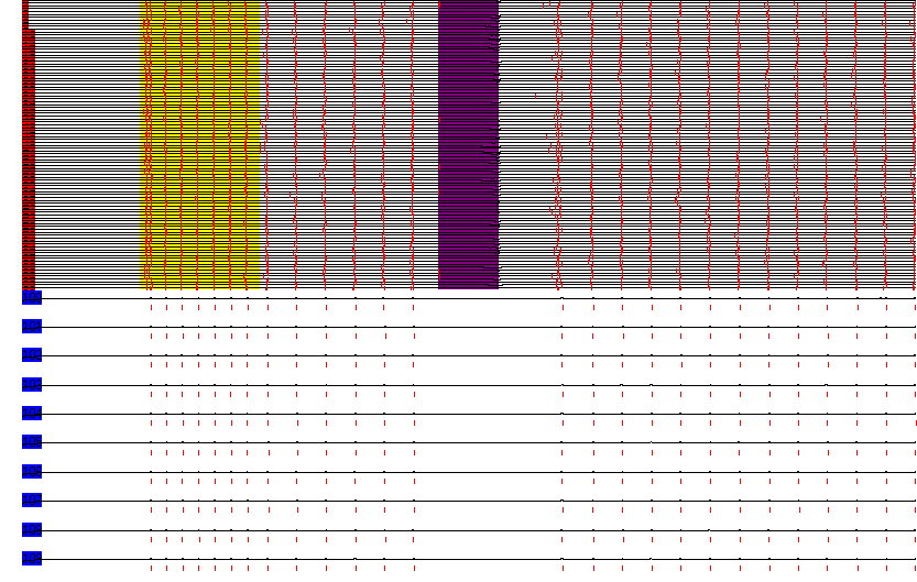
Each line depicts the time-course of the membrane potential of a neuron. The red bars indicate a spike. Neurons with a red label are part of an interconnected excitatory set. The blue labels indicate neurons in an inhibitory set excited by the excitarory set, and sending recurrent inhibition back to it.The region in yellow reflects external activation to the excitatory set, initiating the oscillation. The purple region indicates external inhibition, showing that the oscillation can resurrect even after the absence of spikes for much longer than a period of the oscillation. The behaviour results from slow excitatory membrane dynamics interacting with inhibitory feedback.
Someday who knows, maybe actually use the language / environment to do more than toy-modelling =)
Manual for Rocky 3
1. Introduction
Rocky 3 simulates networks of spiking neurons based on the membrane and synaptic dynamics of biological neurons. Rocky 3 can be used via script files containing commands that specify the architecture of a network and the stimulation to be applied to it.1.1 Neuron and synapse models
These are taken from Wang; the acceptable ranges for parameters can be taken from neuroanatomical data. An essential aspect of network function is the random input to neurons. This is specified as a Poissonian spike input, with a simple decay function associated with random spikes, plus a constant input current. Suitable random input is necessary to keep neurons just under their firing threshold, so that they will be sensitive to network activity. Without random input, it will be very hard to pull a neuron's membrane potential from the leakage voltage up to the firing threshold.1.2 Network architecture
The neurons in a rocky 3 network are connected based on a flexible modular scheme. Each module, i.e. group of neurons, consists of a certain number of excitatory and inhibitory neurons. Each member neuron is connected to each other neuron via a suitable synapse - AMPA or NMDA for excitatory, GABA for inhibitory neurons - with a chance specified per synapse type. The effect of synaptic connections are weighted by a real number, again specified per synapse type. Neurons belonging to different modules have chances and weights specified per from-module, to-module and synapse type. For example:- module 1: 10 excitatory neurons, all-to-all connectivity for AMPA and NMDA, weighting 0.1.
- module 2: 2 inhibitory neurons, no internal connectivity.
- module 1 to module 2: all-to-all AMPA connectivity, weighting 0.1.
- module 2 to module 1: all-to-all GABA connectivity, wieghting 0.5.
1.3 Network stimulation
The stimulation command specifies to which module current will be applied, how many stimulation events will occur, when they start and stop, and how many nA input they will inject into receiving neurons. These are always the excitatory neurons of the module. Another form of stimulation is oscillatory stimulation: short periods of stimulation are presented with a certain frequency, period length and strength.2. Script and online commands
The commands needed for specifying a network and its stimulation are explained below, together with their mnemonic and syntax. Commands should be entered in the order in which they are presented below: t, mod, arch, weight, stim / oscstim, run. This is because some later commands use information specified by earlier commands.Scripts can be run using the script scriptname command in the Rocky 3 command line. The default script, script.txt in the same directory as rocky3.exe, can be run using the "Run script.txt" button. Commands can also be entered directly in the command line, but scripts are more suitable for defining networks.
Every command line in the script must be ended by an enter, or it will not be processed. Hence, take care with the final run command: make sure that the cursor is able to get to the line below the run-command line in your text editor.
An example of a script using the commands explained below is:
// script script_circMotInt.txt
t 10000 10000
net 2 3
mod 6 0 0 0 0 0 0 0 0 0 50 0 50 0 50 0 0 50 50 0 50 0
arch 0 0 0 0 0
arch 1 1 0 0 0
arch 2 2 1 1 0
arch 3 3 0 0 0
arch 4 4 0 0 0
arch 5 5 0 0 0

// circle
arch 0 1 1 1 0
arch 1 2 1 1 0
arch 2 3 1 1 0
arch 3 0 1 1 0

// oscillator
arch 2 3 1 1 0
arch 3 2 0 0 1

// interference
arch 2 1 1 1 0

delay 0 1 10 0
delay 1 2 10 0
delay 2 3 10 0
delay 3 0 10 0

script gScript.txt

normweights
a 2500 0.06 0 2 2000 0.04 0.0 2
stim 0 1 500 1500 0.3
stim 2 1 4000 6000 0.3
run test
with gScript.txt containing
g 0 0 0 0.075 0
g 0 0 1 0.075 0
g 0 0 2 0 0
g 0 1 0 0.02 0
g 0 1 1 0.02 0
g 0 1 2 0 0
g 1 0 0 0 0
g 1 0 1 0 0
g 1 0 2 0.1 0
gL 0 0.025 0
gL 1 0.02 0
2.1 t(ime specification)
- t N(samples) sampling_frequency
2.2 net(work defaults)
- net N(neuron types) N(synapse types)
2.3 mod(ule specification)
- mod N(modules) p(in){1...st} p(next){1...st} p(out){1...st} N(excitatory in module 1) N(inhibitory in module 1) N(exc in mod 2) N (inh in mod 2) ... (N inh in mod m)
N(modules) specifies how many modules will be defined. There are 3 * N(synapse types) variables of the kind p(.){1...st}. p(in), (next) and (out) specify, for each synapse type, the connection chance between neurons in the same module, from a neuron in module i to a neuron in module i + 1, and between neurons in modules that are neither the same nor neighbouring. If a more specific network architecture is required, the (usually 9) generic connection chances should all be set to zero or one, and deviant connections can be adjusted with subsequent arch (see below) commands.
After the generic connection chances, the number of excitatory and inhibitory neurons should be provided for each module. The nesting structure is the same if more than two neuron types are used (which will require reprogramming the software): for all modules, the N(neurons) for all neuron types should be specified. For example, if there a two neuron types and three modules, each containing 4 excitatory and 1 inhibitory neuron except for module 3, which contains no inhibitory neurons, the syntax would be 4 1 4 1 4 0 4 1.
The weights of connections going from neurons in each module is set to 1 by default. The commands weight and normweights can be used to change the strength of connections.
2.4 arch(itecture)
- arch mod1 mod2 p{1...st}
2.5 g(, i.e. conductance), gL (leakage conductance)
- g fromType toType synapseType mean_conductance sd_conductance
- gL neuronType mean(leakage) SD(leakage)
The gL command sets the leakage conductance for each neuron type in an analogous fashion.
2.6 delay
- delay fromMod toMod synapseType delay[msec] sd[msec]
2.7 weight
- weight mod1 mod2 w{1...st}
weight 1 0 0 0 0.05
would be given (if normweights (see below) is not used). By default, all weights are either zero or one, depending on the consequences of arch commands.
2.8 normweights
This command normalizes all weights based on the number of synapses that converge on a neuron. Each weight is divided by this number, for each synapse type separately.2.9 stim(ulation)
- stim module N(events) start{event 1} stop{event 1} strength{event 1} start{event 2} stop{event 2} strength{event 2} ...
2.10 oscstim(ulation)
- oscstim module N(frequencies) freq{1} pulse duration{1} strength{1} freq{2} pulse duration{2} strength{2} ...
2.11 r(un)
- run savename
2.12 plot
- plot sampleStart sampleEnd moduleStart moduleEnd
2.13 saveplot
- saveplot savename
2.14 Efficient scripting
If you want to test the effects of different arcitectures or stimulations, you can define independent modules that undergo the desired effects, or include multiple definition - run sequences, using different save names. Note that the first method may be impractical because the simulation may become slow or demand too much memory.3 Output
See 2.11 for output files. The plot provided after a run command contains, from top to bottom, the modules, and within them, the time series of the neurons per neuron type (first excitatory, then inhibitory). Spikes are plotted as red lines, positive stimulation as a yellow bar, negative stimulation as a purple bar. The membrane potentials are plotted in black.